Tiny Transformer Learns Modular Reversal
From Zero to (Mechanistic) Interpretability
This is a gentle introduction to Transformers and Mechanistic Interpretability. We will build up a simple toy problem, train a tiny Transformer and try to understand its internals using TransformerLens. We will start by introducing transformers and their top level components, discuss how to train them, and then analyze the trained model. Additionally, we will do a very basic ablation to show that both the MLP layer and attention mechanism of a transformer is required for our non-linear problem.
Transformers as Autoregressive Models
Transformers are statistical models for predicting the next token in a sequence, often described as learning a probability distribution. The “context” is whatever tokens have appeared so far, and the model tries to output the distribution over what the next token might be. This is known as autoregressive prediction: the model picks one token at a time, then includes that prediction in its context for predicting the next token, and so on.
In modern language modeling, the context might be hundreds or thousands of tokens (like the words in an article) and the vocabulary might be in the tens of thousands of tokens. In this tiny example, we only have 17 tokens per sequence and a vocabulary of 5. But the same mechanism applies: at each position, the Transformer tries to figure out “which token is most likely next?” given all the tokens that came before.
Detour: The Transformer Architecture
Before we begin with our experiment, we should have some top-level understanding of the transformer architecture. If you are familiar with the topic, you can skip to the next section.
If you want a deeper understanding about this topic, I recommend Neel Nanda’s What is a Transformer? series. Especially the first video is highly helpful for understanding Transformers at a high-level.
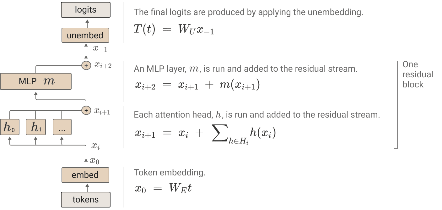
Here is the transformer architecture:
` `
` `
- Token Processing
- Tokenization: Input text is converted to integer tokens from a vocabulary (dimension
vocab_size) - Embedding: Tokens are transformed into vectors in the model’s hidden space (dimension
d_model)
- Tokenization: Input text is converted to integer tokens from a vocabulary (dimension
- Transformer Layers (the model’s processing core, repeated N times)
- Each layer consists of an attention block and an MLP block
- Both blocks connect to the residual stream, allowing information to flow through the network
- Attention Layer
- Helps the model decide which part of the input should be attended to when producing the current output. Attention layers are usually split into multiple attention heads, and the input is split evenly between heads.
- Feed-Forward Network (MLP)
- Two-layer network with non-linear activation. Takes the residual stream and applies the non-linear transformations.
- Output Processing
- Unembedding: Final representations are linearly projected to the vocabulary size.
- Softmax: Converts logits to a probability distribution over the vocabulary.
Motivation: A Simple Task That Requires Both Attention & Non-Linear Processing
We want a toy problem that is neither trivial nor so complicated that interpretability becomes daunting. It’s good to recall that purely linear tasks are generally straightforward and don’t require the fancy machinery of Transformers. For instance, if you had a linear function mapping inputs to outputs (like applying a matrix multiplication), a single linear layer could solve it without needing multi-head attention or multiple layers.
A classic small example is the XOR problem in machine learning. XOR is famously not linearly separable, so a single linear model fails. You need at least a non-linear function to solve XOR. This is a clue that non-linearity can be essential for even small but “interesting” tasks.
In our case, we want to combine two components of complexity: reversal (which we can think of as a kind of “routing” or “token rearrangement,” well suited to attention) and incrementing mod 4 (a small arithmetic shift that’s effectively a non-linear transformation). If we only had reversal, attention alone could handle it. If we only had incrementing mod 4, we wouldn’t particularly need attention. But if we want both in the same problem, the model has to employ attention to fetch the reversed input token and then apply the feedforward net to increment that token by 1 mod 4.
Hence the final “modular reversal” problem hits a sweet spot: the reversed element is learned via the attention mechanism, and the +1 arithmetic is learned by the feedforward layer. Together, they form a minimal example that forces the Transformer to coordinate attention and non-linear processing.
The Problem: Reverse & Increment (Mod 4)
We feed the model sequences of length 17, structured as:
$[BOS, x_0, x_1, x_2, x_3, x_4, x_5, x_6, x_7, y_0, y_1, y_2, y_3, y_4, y_5, y_6, y_7]$
We have a 5-token vocabulary: $0, 1, 2, 3$ plus a special $BOS$ = 4. The first 9 tokens ($[BOS, x_0, .., x_7]$) are interpreted as input, and the final 8 tokens $(y_0..y_7)$ are the output. Each output token is defined to be the corresponding input token reversed in order, plus 1 mod 4.
Concretely:
| If the inputs are | $[0, 1, 2, 3, 2, 0, 3, 1]$ |
| Then the reversed inputs are | $[1, 3, 0, 2, 3, 2, 1, 0]$ |
| Adding 1 mod 4 gives | $[2, 0, 1, 3, 0, 3, 2, 1]$ |
So the full sequence is:
$[BOS, 0, 1, 2, 3, 2, 0, 3, 1, 2, 0, 1, 3, 0, 3, 2, 1]$
The Transformer is trained as an autoregressive model to predict the next token at each position. We specifically compute loss only on the final 8 tokens, so the model focuses on accurately producing the $y_0$..$y_7$ region.
Generating All Possible Sequences
A useful twist in this toy setup is since we have 8 total $x_i$ with 4 different values, there are $4^8 = 65,536$ possible input sequences in total. We easily generate them all and append each sequence’s output. We then shuffle and split 60,000 sequences for training and 5,536 for holdout. Since our holdout set is large and covers many combinations, we do not have to worry about overfitting. If the Transformer learns a genuine circuit, it should do perfectly on the holdout set too.
# Generate all 4^8 possible input sequences.
all_sequences = list(itertools.product(range(4), repeat=8))     #  65536 sequences
all_sequences = torch.tensor(all_sequences, dtype=torch.long)   # shape [65536, 8]

# Compute targets: reverse the sequence and add 1 mod 4.
targets = torch.flip((all_sequences + 1) % 4, dims=[1])         # shape [65536, 8]

# Prepend BOS token (4)
BOS_TOKEN = 4
BOS_column = torch.full((all_sequences.size(0), 1), BOS_TOKEN, dtype=torch.long)

# Concatenate to get full sequence: [BOS, x0..x7, y0..y7] with shape [65536, 17]
full_dataset = torch.cat([BOS_column, all_sequences, targets], dim=1)

# Split into training and holdout sets.
train_dataset = full_dataset[:60000]
holdout_dataset = full_dataset[60000:]
A Tiny Transformer Configuration
We define a miniature Transformer architecture:
$n_{layers} = 1,$ $d_{model} = 4,$ $d_{head} = 4,$ $n_{heads} = 1,$ $d_{mlp} = 16,$ $d_{vocab} = 5,$ $n_{ctx} = 17.$
cfg = HookedTransformerConfig(
    n_layers=1,
    d_model=4,         # Hidden dimension
    d_head=4,          # Head dimension
    n_heads=1,         # One head for simplicity
    d_mlp=16,          # MLP hidden dimension
    d_vocab=5,         # Vocabulary: tokens 0,1,2,3, BOS (4)
    n_ctx=17,          # Sequence length (BOS + 8 in + 8 out)
    act_fn='relu',
    normalization_type='LN',
    device='cuda' if torch.cuda.is_available() else 'cpu'
)
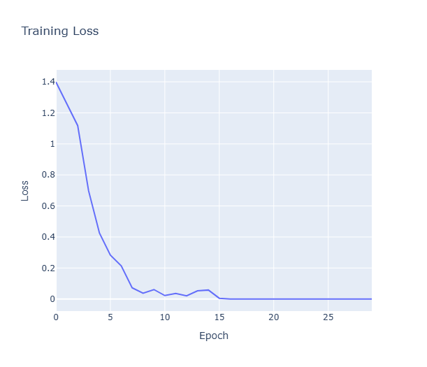
We train it for 30 epochs with gradient clipping and a cosine decay learning rate schedule. The model trains quickly and eventually hits 100% accuracy on the holdout set. We keep and evaluate on an holdout set to see whether the current accuracy is due to memorizing from the seen data or it is truly generalizing to unseen sequences as well.
In traditional ML evaluation, models are often treated as black boxes, caring only about input-output behavior. Mechanistic interpretability wants to understand how the model works internally in a bottom-up approach. One research interest in MI is about how the smallest building blocks in models compose together to produce circuits (hypothesis is that the models learn circuits to implement algorithms.) In this fashion, let’s try to interpret some parts of our modest model!
In our tiny transformer, we’ll examine how the model works internally by analyzing:
- How attention routes information from inputs to outputs
- How the MLP transforms representations
- How these components combine to solve our reversal + increment task
Peeking Under the Hood: Attention Patterns
Attention is the mechanism that allows transformers to gather information from other positions. For our task, the attention mechanism should learn to focus on the reversed positions in the input.
Let’s examine the attention patterns for each output position:
# Run model with cache to capture intermediate activations
sample = holdout_dataset[:4].to(device)  # 4 example sequences
logits, cache = model.run_with_cache(sample[:, :-1])

# Extract attention patterns
attn = cache["pattern", 0]  # shape: [batch, n_heads, 16, 16]

# Look at attention from output positions (8-15) to input positions (1-8)
attn_target = attn[:, :, 8:, 1:9]  # shape: [4, 1, 8, 8]
Using plotly, here is the visualization of our attention matrix between $x_i$ and $y_i$:

Look at the diagonal! For each output position, the attention strongly focuses on precisely one input position. For example, the first output position (y0, index 8) attends almost exclusively to the last input position (x7, index 8). Similarly, the second output position attends to the second-to-last input, and so on.
Of course, we can inspect the attention matrix directly as well. Here is one sample where we can see the diagonal again:
[[4.42e-04 1.41e-03 4.61e-07 1.47e-08 4.53e-02 6.60e-06 2.12e-09 9.53e-01]  y0 -> x7
 [4.56e-05 3.08e-05 1.98e-03 4.61e-02 3.87e-08 8.63e-04 9.35e-01 5.88e-10]  y1 -> x6
 [2.37e-02 4.54e-07 2.21e-01 1.93e-03 2.31e-13 6.33e-01 3.46e-10 3.44e-12]  y2 -> x5,x3
 [1.25e-10 3.79e-06 1.02e-12 2.97e-11 9.04e-01 1.54e-12 3.45e-05 9.57e-02]  y3 -> x4
 [3.93e-15 3.13e-17 1.94e-05 2.13e-03 4.94e-11 1.16e-10 5.52e-05 1.39e-09]  y4 -> x3
 [2.10e-12 2.20e-18 6.52e-02 8.35e-02 2.97e-16 6.60e-07 2.82e-09 2.59e-13]  y5 -> x2,x3
 [1.18e-05 9.04e-01 6.90e-19 1.42e-20 1.53e-06 3.84e-12 2.44e-15 3.60e-09]  y6 -> x1
 [8.97e-01 2.11e-03 5.51e-06 2.17e-08 3.95e-15 5.19e-02 3.25e-12 2.60e-16]] y7 -> x0
This pattern is what we’d expect for the reversal task! Each output position is attending to the corresponding input position in reverse order. The model has learned the correct routing pattern to fetch the right input tokens.
Looking at multiple examples from our holdout set, we see this pattern is pretty consistent. The attention mechanism has learned to handle the reversal part of our task.
MLP: The Non-Linear Transformation
Once the attention mechanism has routed the proper token to each position, the MLP needs to transform it by adding 1 mod 4. We can directly examine the MLP output tensor by:
# Extract MLP outputs
mlp_out = cache["mlp_out", 0]  # shape: [batch, 16, d_model]
However, MLP outputs are harder to interpret directly, so we’ll compare the final hidden states with the embeddings for each token:
def compare_to_embeddings(model, data, n_examples=4):
    # After attention but before MLP
    attn_out = cache["attn_out", 0]  # shape: [batch, seq_len, d_model]
    resid_pre = cache["resid_pre", 0]  # shape: [batch, seq_len, d_model]
    attn_plus_residual = attn_out + resid_pre  # shape: [batch, seq_len, d_model]

    # MLP output
    mlp_out = cache["mlp_out", 0]  # shape: [batch, seq_len, d_model]

    # Compare these with the unembedding matrix (final projection)
    unembed = model.unembed.W_U  # shape: [d_vocab, d_model]

    # Project activations to logits
    pre_mlp_logits = attn_plus_residual @ unembed  # Before MLP contribution
    post_mlp_logits = (attn_plus_residual + mlp_out) @ unembed  # With MLP

    # Look at a specific example
    idx = 0  # First example
    for pos in range(8, 16):  # Output positions
        input_pos = 16 - pos  # Reversed position (due to 1-indexing offset)
        input_token = sample[idx, input_pos].item()
        expected_output = (input_token + 1) % 4

        # Get activation logits at this position
        pre_mlp = pre_mlp_logits[idx, pos, :5].cpu().numpy()
        post_mlp = post_mlp_logits[idx, pos, :5].cpu().numpy()

        # Convert to probabilities
        pre_probs = F.softmax(torch.tensor(pre_mlp), dim=0).numpy()
        post_probs = F.softmax(torch.tensor(post_mlp), dim=0).numpy()

        print(f"Position {pos} (input={input_token}, expected={expected_output}):")
        print(f"  Before MLP: {pre_probs} (argmax={pre_mlp.argmax()})")
        print(f"  After MLP:  {post_probs} (argmax={post_mlp.argmax()})")
Let’s look at the results for our first example:
=== Sample 0 ===
Sequence: [4, 3, 2, 2, 2, 1, 2, 0, 0, 1, 1, 3, 2, 3, 3, 3, 0]
Position 8 (input=0, expected=1):
  Before MLP: [8.0037588e-10 9.9641526e-01 1.7016100e-07 3.5106475e-03 7.3987991e-05] (argmax=1)
  After MLP:  [2.4150684e-09 9.9913752e-01 4.5021100e-08 7.2877557e-04 1.3367768e-04] (argmax=1)
# ...
Position 11 (input=1, expected=2):
  Before MLP: [0.47883704 0.07598887 0.07476649 0.05180051 0.3186071 ] (argmax=0)
  After MLP:  [0.00237166 0.00099805 0.6154633  0.37624195 0.00492504] (argmax=2)
# ...
Position 13 (input=2, expected=3):
  Before MLP: [0.6005856  0.10933079 0.11232433 0.03671417 0.14104511] (argmax=0)
  After MLP:  [2.7413596e-04 2.6834223e-02 2.2894813e-02 9.4326144e-01 6.7354082e-03] (argmax=3)
# ...
Position 15 (input=3, expected=0):
  Before MLP: [8.5525554e-01 3.1973116e-06 1.3825244e-01 2.7612159e-03 3.7276892e-03] (argmax=0)
  After MLP:  [9.5289975e-01 2.0124548e-05 4.0074017e-02 3.4347910e-04 6.6626580e-03] (argmax=0)

argmaxes = [1, 1, 3, 2, 3, 3, 3, 0]
Note: Understanding the Pre-MLP State
To avoid any confusion about the output just presented, we need to understand what’s happening in the transformer’s residual stream. At each output position, the pre-MLP state (attn_plus_residual) is a combination of:
- The original embedding at that position (
resid_pre) - The output from the attention layer (
attn_out), which contains information gathered from input positions via attention
The attention mechanism doesn’t perfectly extract the pure embedding of the input token it’s attending to. Rather, it produces a weighted sum of value vectors from all positions (heavily weighted toward the reversed input position). When we project this mixed representation to logits (via the unembedding matrix), we don’t necessarily get a clean prediction matching the attended token. This is why some pre-MLP states show strong predictions for tokens other than what we’d expect from the attention pattern alone. The MLP’s job is to transform this mixed representation to produce the correct “+1 mod 4” token.
With that out of the way, let’s look at our expected answer and what is outputted as the most likely token from the MLP layer:
- Input:
[3, 2, 2, 2, 1, 2, 0, 0](after BOS) - Reversed:
[0, 0, 2, 1, 2, 2, 2, 3] - +1 mod 4:
[1, 1, 3, 2, 3, 3, 3, 0] - argmaxes:
[1, 1, 3, 2, 3, 3, 3, 0]
We can clearly see that MLP is indeed performing the “+1 mod 4” transformation. It’s working as a non-linear function that takes the pre-MLP residual stream and adds back to the residual stream to steer the final output to the correct output token representation.
With the results from Attention layer and the MLP layer, we have a strong understanding of how the layers perform their respective operations. Finally, for educational purposes, let’s also do some basic ablations.
Ablation: Verifying Both Parts Matter
To confirm our mechanistic understanding, let’s perform a simple ablation study. If our hypothesis about the circuit is correct, then disabling either the attention or MLP components should break the model’s ability to solve the task.
def ablate_linear_weight(tensor: torch.Tensor):
    """Zero out the given weight tensor in-place and return a backup copy."""
    backup = tensor.detach().clone()
    with torch.no_grad():
        tensor.zero_()
    return backup

# 1) Ablate MLP output weights
backup_wout = ablate_linear_weight(model.blocks[0].mlp.W_out)
acc_after_mlp_ablation = evaluate_model(model, holdout_dataset)
print(f"After zeroing MLP W_out, holdout accuracy: {acc_after_mlp_ablation*100:.2f}%")
model.blocks[0].mlp.W_out.data.copy_(backup_wout)

# 2) Ablate Attention output
backup_wo = ablate_linear_weight(model.blocks[0].attn.W_O)
acc_after_attn_ablation = evaluate_model(model, holdout_dataset)
print(f"After zeroing Attention W_O, holdout accuracy: {acc_after_attn_ablation*100:.2f}%")
model.blocks[0].attn.W_O.data.copy_(backup_wo)
The results confirm our hypothesis:
- Original accuracy: 100.00%
- Accuracy after zeroing MLP $W_{out}$: 17.67%
- Accuracy after zeroing Attention $W_0$: 29.19%
Disabling either component drastically reduces performance, showing that both are essential for the task. Interestingly, zeroing the attention has a more severe effect than zeroing the MLP. I assume their accuracies would have been closer if we had computed accuracy on the whole distribution instead of just evaluating on the limited holdout samples.
Putting It All Together: The Complete Circuit
Let’s synthesize our findings into a complete picture of how our single-layer transformer solves the modular reversal task:
-
Input Processing: Each token (including the BOS token) gets embedded into a 4-dimensional vector.
-
Attention Routing: For each output position
y_i, the attention mechanism learns to focus almost exclusively on the corresponding reversed input positionx_{7-i}. This effectively implements the reversal part of the task by routing the correct token’s information. -
MLP Transformation: Once the attention mechanism has routed the input token’s information, the MLP applies a non-linear transformation that shifts the representation to be closer to the token value + 1 mod 4.
-
Final Prediction: The transformed representation is then fed through the unembedding matrix to produce logits, with the highest logit corresponding to the correct output token.
This circuit neatly divides the task between the attention mechanism (handling reversal) and the MLP (handling the increment). It’s a clean example of how transformer components can specialize to handle different aspects of a problem.
Conclusion
Even this tiny transformer uses the same fundamental approach as large language models: it forms an autoregressive distribution and uses attention to figure out which tokens matter for each position, then applies a non-linear transformation in the MLP to finalize its output. Our toy example was designed so that reversal alone (which is basically “linear routing”) is insufficient without a +1 mod 4 shift, and that shift is insufficient without retrieving the reversed input. By combining both, we see that attention and feedforward layers jointly solve the task.
Through mechanistic interpretability, we’ve peered inside the “black box” and verified exactly how our transformer solves the task. In real life, transformer models are huge and it is impractical to search for circuits by hand. However, I hope that this experience was fun and useful as a way to understand how small models can be inspected to understand their behaviour.
Addendum
This article was written for BlueDot’s AI Safety Course and Neel Nanda’s resources were invaluable. If this small project piques your interest in mechanistic interpretability, you should definitely check out Neel Nanda through his blog and YouTube channel to get a more in-depth exploration of transformers and mechanistic interpretability.